Let us traverse the trie (see fig 4.2) with the postorder method and see how the partition can be performed. We start with the (lexicographically) first leaf. All states up to the first forward-branching state (state with more than one outgoing transition) must belong to different classes. We can put them into a register of states so that we can find them easily. There will be no need to replace them by other states. Looking at the next branches, and starting from their leaves, we first need to know whether a given state belongs to the same class or not. Newly considered states belong to the same class as a representative of an established class if and only if:
The last condition is satisfied by the postorder method used to traverse the trie. If all the conditions are satisfied, the state is replaced by another state found in the register. If not, then it must be a representative of a new class, so it must be put into the register.
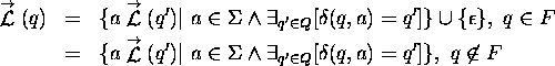
This procedure leads to a minimal automaton . Note that all leaves belong to the same class. If a pair of states have equivalent transitions (the same number of transitions, with the same labels, and the same target states), and if the target states are the sole representatives of their classes, then the right language of each pair of target states is the same. Hence our intuition about equivalence of states is supported by our alternate definition of minimal automata .
All leaves have the same right language, {![]() }, which is the
empty string. If any pair of states have the
same right language, then that language can be represented as
}, which is the
empty string. If any pair of states have the
same right language, then that language can be represented as
Note that this is simply the inductive definition of the right
language of a state (using ![]() instead of
instead of ![]() ). This
confirms that the states must have an equal
number of transitions that have the same labels, and lead to states
that have the same right languages. They also must be both either
final, or non-final (the difference between final and non-final states
is that the final ones have
). This
confirms that the states must have an equal
number of transitions that have the same labels, and lead to states
that have the same right languages. They also must be both either
final, or non-final (the difference between final and non-final states
is that the final ones have ![]() in their right language).
in their right language).
Now we want to add new words to our automaton gradually while
maintaining the minimality property . We need to know
how to synchronize two processes: one that adds new words to the
automaton, the other that minimizes it. There are
two crucial questions to be answered. Firstly, which states are
subject to change when new words are added? Secondly,is there a way to
add new words to the automaton such that we minimize the number of
states that may need to be changed during the addition of a word?
Looking at the figures 4.2 and 4.3,
it becomes clear that in order to reproduce the same order of
traversal of states, the data must be lexicographically sorted. Note
that in order to this, ![]() must be ordered. Farther investigation
reveals that when we add words in this order, only the states that
need to be traversed to accept the last word added to the automaton
may change when words are added. All the rest of the automaton remains
unchanged. This happens because states are changed by removing them or
by appending new transitions. We call a common
prefix the longest prefix of the new word that
is also a prefix of a word already in the automaton. New transitions
can only be added to the last state that belongs to the common
prefix of new word added to the automaton. Since the words are
lexicographically sorted, the common prefix can contain only states
that represent the beginning of the last word added to the automaton
(the whole word if the last word is a prefix of the new word). Each
new word can either reuse the states from the common prefix, or it can
add new states. The states may be removed only from the path that
represents the last word added to the automaton (the part that does
not contain the common prefix). When a new word is added, and the last
word is not a prefix of the new word, then states in that part are
subject to either removal (they are replaced by other identical
states) or they are registered as new states. That discovery leads us
to the algorithm given in fig 4.4.
must be ordered. Farther investigation
reveals that when we add words in this order, only the states that
need to be traversed to accept the last word added to the automaton
may change when words are added. All the rest of the automaton remains
unchanged. This happens because states are changed by removing them or
by appending new transitions. We call a common
prefix the longest prefix of the new word that
is also a prefix of a word already in the automaton. New transitions
can only be added to the last state that belongs to the common
prefix of new word added to the automaton. Since the words are
lexicographically sorted, the common prefix can contain only states
that represent the beginning of the last word added to the automaton
(the whole word if the last word is a prefix of the new word). Each
new word can either reuse the states from the common prefix, or it can
add new states. The states may be removed only from the path that
represents the last word added to the automaton (the part that does
not contain the common prefix). When a new word is added, and the last
word is not a prefix of the new word, then states in that part are
subject to either removal (they are replaced by other identical
states) or they are registered as new states. That discovery leads us
to the algorithm given in fig 4.4.
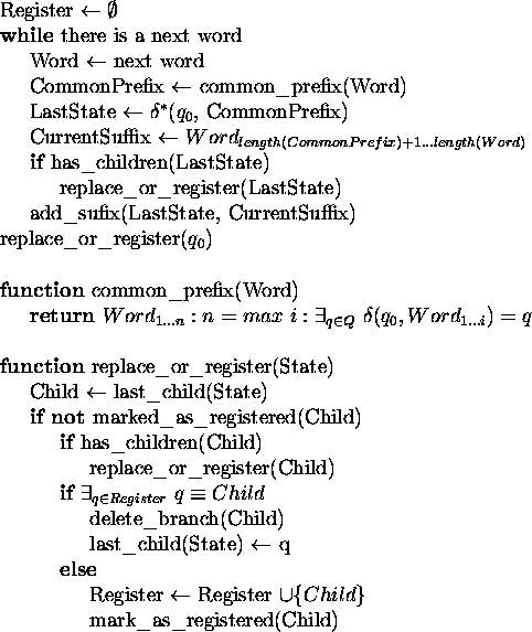
Figure 4.4: Incremental construction algorithm for sorted
data
The function common_prefix finds the longest prefix (of the word to be added) that is a prefix of a word already in the automaton.
The function add_suffix creates a branch extending out of the automaton that represents the suffix of the word being added (the portion of the word which is left after the common prefix has been cut). The last state of this branch is marked as final. The function last_child returns the state reached by the (lexicographically) last transition which is going out from the argument state. Since the data is lexicographically sorted, last_child returns the state reached by the transition added most recently from the state (during the addition of the previous word). Each state has a marker that indicates whether or not it is already registered, because it is necessary to determine which states have already been processed. Some parts of the automaton are left for further treatment (replacement or registering) until some other word is added so that those states no longer belong to the path in the automaton that accepts the new word.. That marker is read with marked_as_registered, and set with mark_as_registered. Finally, has_children returns true if there are outgoing transitions from the state, and delete_branch deletes its argument state and all states that can be reached from it (if they are not already marked as registered).
Memory requirements for this algorithm are at the maximum towards the end of processing. Memory is needed for the minimized automaton that is under construction, the call stack, and for the register of states. The memory for the automaton is proportional to the number of states and the total number of transitions. The memory for the register of states is proportional to the number of states, and can be freed once the construction is complete.
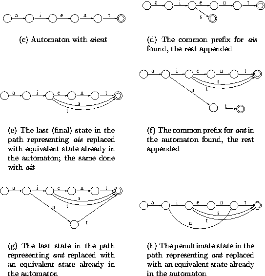
Figure 4.5: Examples of construction process for sorted data
The main loop of the algorithm runs m times, where m is the number
of words to be accepted by the automaton. The function common_prefix
executes in ![]() time, where |w| is the maximum word
length. The function replace_or_register executes recursively at
most |w| for each word. In each recursive call, there is one
register search, and there may be one register insertion. The
pessimistic time complexity of the search is
time, where |w| is the maximum word
length. The function replace_or_register executes recursively at
most |w| for each word. In each recursive call, there is one
register search, and there may be one register insertion. The
pessimistic time complexity of the search is ![]() ,
where n is the number of states in the (minimized) automaton. The
pessimistic time complexity of adding a state to the register is also
,
where n is the number of states in the (minimized) automaton. The
pessimistic time complexity of adding a state to the register is also
![]() . By using a hash table to represent the
register, the average time complexity of those operations can be made
constant. Since all children of a state are either replaced or
registered, delete_branch executes in constant time. So the
pessimistic time complexity of the entire algorithm is
. By using a hash table to represent the
register, the average time complexity of those operations can be made
constant. Since all children of a state are either replaced or
registered, delete_branch executes in constant time. So the
pessimistic time complexity of the entire algorithm is
![]() , while an average time complexity of
, while an average time complexity of
![]() can be achieved.
can be achieved.
Figure 4.5 shows examples of the construction process for data: aient, ais, ait and ant.