 ).
).
The size of the automaton, and the speed of its use, depend on the method used for its representation. The differences can be drastic. It should be noted that there is no single representation method suitable for all applications and providing the best characteristics in all aspects. The choice must be seen as a compromise between various requirements. The representations of automata are the same as those for directed graphs (see e.g. [AHU74]).
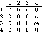
Two classical methods are the neighborhood
matrix and lists. The neighborhood
matrix is a matrix where one axis is labeled with the source state
numbers of the transitions, and the other one is labeled with the
target state numbers of the transitions. State attributes must be
stored elsewhere, i.e. in another vector. The entries in the matrix
are the attributes of the transitions, here:
labels. Table 4.1 shows such a structure for the
example automaton from fig. 2.3
(page  ).
).

Table: Neighborhood matrix for example automaton from
fig. 2.3
As large automata may have millions of states, and there may be many different transitions between states, such method cannot be effective. A variant of the neighborhood matrix uses all possible symbols as the columns; the target states are values of the matrix. Such matrix is much better than the previous one, both in terms of memory requirements and processing time.
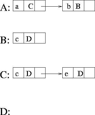
Another traditional approach is to use coincidence
lists. Fig. 4.10 shows the example automaton from
fig.2.3 (page  ) in form of
coincidence lists.

Figure: Example automaton from fig. 2.3 represented by lists
Note that if the transitions can be stored in consecutive memory locations, then there is no need for links to the next transitions. What is needed is the number of transitions for the state. Transitions can be stored as consecutive entries in a vector. If we move the properties: the number of transitions, and the final status of the states to the transitions that lead to them, we no longer need to store the states explicitly; they will be stored implicitly in the transitions. See table 4.2 for an example. Interestingly, moving some state properties to transitions resulted in the creation of a new state. That state exists solely because its dummy transition provides the properties of the initial state.

Table: Example automaton from fig.2.3
represented by vectors of transitions
Since the states in the method shown above are implicit, further compression is possible. Two such methods were explored in the implementation of the automata construction algorithms presented in this dissertation:
Note that for the first method to work efficiently, the transitions
should be sorted. The order imposed by the sorting affects
compression. The best results can be achieved by sorting the
transitions on the frequency of occurrences of their
labels . Finding the ideal layout of the transitions in each state is
NP-hard. Table 4.3 shows the example automaton
where one of states (B) was put into another state (C). Assuming that
all transitions of a state are ordered, we denote as
![]() the ith transition of the state q. For a given
state
the ith transition of the state q. For a given
state ![]() , the method consists in finding a representation of a
state
, the method consists in finding a representation of a
state ![]() such that
such that
![]()

Table: Example automaton from fig. 2.3
represented by vectors of transitions - state B resides inside
state C
The other method can be applied after the first one described
above. We take a state represented as a set of its outgoing
transitions and look for two other states. A few of the last
transitions of first one should be the same as the first transitions
of the state we want to compress, and the remaining transitions of the
state to be compressed should be the same as the first transitions of
the second state we search for. Formally, for a given state ![]() , we
look for states
, we
look for states ![]() and
and ![]() such that
such that ![]() and
and ![]() , and
, and ![]() , and:
, and:
![]()
and
![]()
In our programs all states that were allowed to take part in such match-making had two transitions.
Tomasz Kowaltowski ([KLS93b]) uses a form of coincidence lists to obtain the best compression of automata. A state of a traditional finite-state automaton is treated as a list of states of a binary automaton . Those states (we will call them binary states here to avoid confusion with the states of a traditional FSA) correspond to the transitions of the traditional FSA. Each state of the binary automaton has two pointers. The first one leads to the target state of the transition. The second one points to the next transition in the current state of the original FSA. Tomasz Kowaltowski notes that, with such representation of states, it is possible to merge the endings of two lists, i.e. to merge parts of states. Note that in the approach described above, a state can be merged either with two adjacent states, or with only one bigger state that contains all transitions of the smaller state (that bigger state may further be merged with an even bigger state). In Kowaltowski's approach, one smaller state may be merged with several bigger states that cannot be merged one into another.
A proper state is a binary state that is either:
Proper states are visited in order so that a proper state cannot be visited before all proper states that are targets of the transitions of that state are visited. When a proper state is visited, one looks among all states already visited for a state that contains a set of binary states being a subset of the set of transitions of the current state. From the set of states found in that search the state with the biggest number of binary states is chosen. The binary states in the current proper state are reordered so that those that are present in the chosen state are in the end. Then a pointer to them is replaced with a pointer to the chosen proper state.
To maximize the probability that the current state will be matched by parts of other states, its binary states that are not shared with chosen proper state are ordered by the frequency of their occurrence in the proper states that were not visited yet, and contain the binary states of the chosen state. The failure transition of the least frequent binary state in a proper state points to a more frequent binary state, and so on to the most frequent binary state whose failure transition points to the chosen state.
The automaton is represented as a vector of binary states. Judicious
coding makes it possible to obtain substantial compression. The
symbols (the labels of transitions) are coded on
![]() bits. The number of symbols in the
language is incremented by one to accommodate for a special symbol
that marks the end of the word. Tomasz Kowaltowski notes that most
states of an FSA have only one transition, and thus the target of that
transition is the previous state (states are numbered from
the sink state up to the start state). An extra bit distinguishes
between the situation when the target is the previous binary state, or
not. In the latter case the target state number i is coded on k bits,
where
bits. The number of symbols in the
language is incremented by one to accommodate for a special symbol
that marks the end of the word. Tomasz Kowaltowski notes that most
states of an FSA have only one transition, and thus the target of that
transition is the previous state (states are numbered from
the sink state up to the start state). An extra bit distinguishes
between the situation when the target is the previous binary state, or
not. In the latter case the target state number i is coded on k bits,
where ![]() . There are no final
states, i.e. no states need to bare the marker of being final, as the
end of the word is marked by a special symbol. This means that every
final state has a transition labeled with that symbol. In that case,
there is no need to code the target state, as it is the same for all
transitions labeled with the symbol.
. There are no final
states, i.e. no states need to bare the marker of being final, as the
end of the word is marked by a special symbol. This means that every
final state has a transition labeled with that symbol. In that case,
there is no need to code the target state, as it is the same for all
transitions labeled with the symbol.
In the case of the failure transition, most target states are either the previous binary state (states are numbered from the end), or none. The third possibility is an arbitrary state (coded as shown above), so it is possible to use one or two bits to distinguish between these 3 situations. Tomasz Kowaltowski reports compression rates (the size of the compressed folded automaton divided by the size of the original automaton) up to 99%.
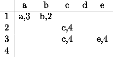
Dominique Revuz ([Rev91]), and Emmanuel Roche and Yves
Schabes ([RS95]) argue for a different representation
method. The automaton is stored in a matrix where each row is a state,
and each column is labeled with one symbol. There are ![]() columns. If a transition from a given state labeled with a given
symbol exists, the entry with the coordinates (state, symbol) contains
that symbol and the number of the target state. Otherwise it contains
something else.
columns. If a transition from a given state labeled with a given
symbol exists, the entry with the coordinates (state, symbol) contains
that symbol and the number of the target state. Otherwise it contains
something else.

Table: Matrix labeled with states and symbols storing the
example automaton from fig. 2.3
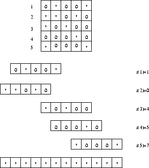
As the example shows, such a table is sparse, so they recommend using
a method described in [TY79]. The method
(fig. 4.11) compresses the matrix by trying to arrange
its rows so that they overlap. The matrix is compressed to a
vector. For each row, an attempt is made to store it in the vector in
such a way that the transitions fall into empty spaces left from other
rows. The empty spaces appear when the state in question does not have
![]() transitions. For each symbol in
transitions. For each symbol in ![]() being the
potential label, if there is no transition labeled with it, an empty
space appears.
being the
potential label, if there is no transition labeled with it, an empty
space appears.

Figure 4.11: Compression of a sparse table (adopted from
[TY79])